`numina.array` — Array manipulation

numina.array.fixpix(data, mask, kind='linear'): Interpolate 2D array data in rows

numina.array.fixpix2(data, mask, iterations=3, out=None): Substitute pixels in mask by a bilinear least square fitting.

numina.array.numberarray(x, shape): Return x if it is an array or create an array and fill it with x.

numina.array.rebin(a, newshape): Rebin an array to a new shape.

numina.array.rebin_scale(a, scale=1): Scale an array to a new shape.

numina.array.subarray_match(shape, ref, sshape, sref=None)

Compute the slice representation of intersection of two arrays.

Given the shapes of two arrays and a reference point ref, compute the intersection of the two arrays. It returns a tuple of slices, that can be passed to the two images as indexes

Parameters:

shape – the shape of the reference array
ref – coordinates of the reference point in the first array system
sshape – the shape of the second array

Param:

sref: coordinates of the reference point in the second array system, the origin by default

Returns:

two matching slices, corresponding to both arrays or a tuple of Nones if they don’t match

Return type:

a tuple

Example

>>> import numpy
>>> im = numpy.zeros((1000, 1000))
>>> sim = numpy.ones((40, 40))
>>> i,j = subarray_match(im.shape, [20, 23], sim.shape)
>>> im[i] = 2 * sim[j]

numina.array.process_ramp(inp[, out=None, axis=2, ron=0.0, gain=1.0, nsig=4.0, dt=1.0, saturation=65631])

New in version 0.8.2.

Compute the result 2d array computing slopes in a 3d array or ramp.

Parameters:

inp – input array
out – output array
axis – unused
ron – readout noise of the detector
gain – gain of the detector
nsig – rejection level to detect glitched and cosmic rays
dt – time interval between exposures
saturation – saturation level

Returns:

a 2d array

`numina.array.background` — Background estimation

Background estimation

Background estimation following Costa 1992, Bertin & Arnouts 1996

numina.array.background.background_estimator(bdata): Estimate the background in a 2D array

numina.array.background.create_background_map(data, bsx, bsy): Create a background map with a given mesh size

`numina.array.blocks` — Generation of blocks

numina.array.blocks.blk_1d(blk, shape)

Iterate through the slices that recover a line.

This function is used by blk_nd() as a base 1d case.

The last slice is returned even if is lesser than blk.

Parameters:

blk – the size of the block
shape – the size of the array

Returns:

a generator that yields the slices

numina.array.blocks.blk_1d_short(blk, shape)

Iterate through the slices that recover a line.

This function is used by blk_nd_short() as a base 1d case.

The function stops yielding slices when the size of the remaining slice is lesser than blk.

Parameters:

blk – the size of the block
shape – the size of the array

Returns:

a generator that yields the slices

numina.array.blocks.blk_coverage_1d(blk, size)

Return the part of a 1d array covered by a block.

Parameters:

blk – size of the 1d block
size – size of the 1d a image

Returns:

a tuple of size covered and remaining size

Example

>>> blk_coverage_1d(7, 100)
(98, 2)

numina.array.blocks.blk_nd(blk, shape)

Iterate through the blocks that cover an array.

This function first iterates trough the blocks that recover the part of the array given by max_blk_coverage and then iterates with smaller blocks for the rest of the array.

Parameters:

blk – the N-dimensional shape of the block
shape – the N-dimensional shape of the array

Returns:

a generator that yields the blocks

Example

>>> result = list(blk_nd(blk=(5,3), shape=(11, 11)))
>>> result[0]
(slice(0, 5, None), slice(0, 3, None))
>>> result[1]
(slice(0, 5, None), slice(3, 6, None))
>>> result[-1]
(slice(10, 11, None), slice(9, 11, None))

The generator yields blocks of size blk until it covers the part of the array given by max_blk_coverage() and then yields smaller blocks until it covers the full array.

`numina.array.bpm` — Bad Pixel Mask interpolation

Fix points in an image given by a bad pixel mask

numina.array.bpm.process_bpm(method, arr, mask, hwin=2, wwin=2, fill=0, reuse_values=False, subs=False)

Parameters:

method –
arr –
mask –
hwin –
wwin –
fill –
reuse_values –
subs –

numina.array.bpm.process_bpm_median(arr, mask, hwin=2, wwin=2, fill=0, reuse_values=False, subs=False)

Parameters:

arr –
mask –
hwin –
wwin –
fill –
reuse_values –
subs –

`numina.array.combine` — Array combination

Different methods for combining lists of arrays.

numina.array.combine.flatcombine(arrays, masks=None, dtype=None, scales=None, low=3.0, high=3.0, blank=1.0)

Combine flat arrays.

Parameters:

arrays – a list of arrays
masks – a list of mask arrays, True values are masked
dtype – data type of the output
out – optional output, with one more axis than the input arrays
blank – non-positive values are substituted by this on output

Returns:

mean, variance of the mean and number of points stored

numina.array.combine.generic_combine(method, arrays, masks=None, dtype=None, out=None, zeros=None, scales=None, weights=None)

Stack arrays using different methods.

Parameters:

method (PyCObject) – the combination method
arrays – a list of arrays
masks – a list of mask arrays, True values are masked
dtype – data type of the output
zeros –
scales –
weights –

Returns:

median, variance of the median and number of points stored

numina.array.combine.mean(arrays, masks=None, dtype=None, out=None, zeros=None, scales=None, weights=None)

Combine arrays using the mean, with masks and offsets.

Arrays and masks are a list of array objects. All input arrays have the same shape. If present, the masks have the same shape also.

The function returns an array with one more dimension than the inputs and with size (3, shape). out[0] contains the mean, out[1] the variance and out[2] the number of points used.

Parameters:

arrays – a list of arrays
masks – a list of mask arrays, True values are masked
dtype – data type of the output
out – optional output, with one more axis than the input arrays

Returns:

mean, variance of the mean and number of points stored

Example

>>> import numpy
>>> image = numpy.array([[1., 3.], [1., -1.4]])
>>> inputs = [image, image + 1]
>>> mean(inputs)
array([[[ 1.5,  3.5],
        [ 1.5, -0.9]],

       [[ 0.5,  0.5],
        [ 0.5,  0.5]],

       [[ 2. ,  2. ],
        [ 2. ,  2. ]]])

numina.array.combine.median(arrays, masks=None, dtype=None, out=None, zeros=None, scales=None, weights=None)

Combine arrays using the median, with masks.

Arrays and masks are a list of array objects. All input arrays have the same shape. If present, the masks have the same shape also.

The function returns an array with one more dimension than the inputs and with size (3, shape). out[0] contains the mean, out[1] the variance and out[2] the number of points used.

Parameters:

arrays – a list of arrays
masks – a list of mask arrays, True values are masked
dtype – data type of the output
out – optional output, with one more axis than the input arrays

Returns:

median, variance of the median and number of points stored

numina.array.combine.minmax(arrays, masks=None, dtype=None, out=None, zeros=None, scales=None, weights=None, nmin=1, nmax=1)

Combine arrays using mix max rejection, with masks.

Inputs and masks are a list of array objects. All input arrays have the same shape. If present, the masks have the same shape also.

The function returns an array with one more dimension than the inputs and with size (3, shape). out[0] contains the mean, out[1] the variance and out[2] the number of points used.

Parameters:

arrays – a list of arrays
masks – a list of mask arrays, True values are masked
dtype – data type of the output
out – optional output, with one more axis than the input arrays
nmin –
nmax –

Returns:

mean, variance of the mean and number of points stored

numina.array.combine.quantileclip(arrays, masks=None, dtype=None, out=None, zeros=None, scales=None, weights=None, fclip=0.1)

Combine arrays using the sigma-clipping, with masks.

Inputs and masks are a list of array objects. All input arrays have the same shape. If present, the masks have the same shape also.

The function returns an array with one more dimension than the inputs and with size (3, shape). out[0] contains the mean, out[1] the variance and out[2] the number of points used.

Parameters:

arrays – a list of arrays
masks – a list of mask arrays, True values are masked
dtype – data type of the output
out – optional output, with one more axis than the input arrays
fclip – fraction of points removed on both ends. Maximum is 0.4 (80% of points rejected)

Returns:

mean, variance of the mean and number of points stored

numina.array.combine.sigmaclip(arrays, masks=None, dtype=None, out=None, zeros=None, scales=None, weights=None, low=3.0, high=3.0)

Combine arrays using the sigma-clipping, with masks.

Inputs and masks are a list of array objects. All input arrays have the same shape. If present, the masks have the same shape also.

The function returns an array with one more dimension than the inputs and with size (3, shape). out[0] contains the mean, out[1] the variance and out[2] the number of points used.

Parameters:

arrays – a list of arrays
masks – a list of mask arrays, True values are masked
dtype – data type of the output
out – optional output, with one more axis than the input arrays
low –
high –

Returns:

mean, variance of the mean and number of points stored

numina.array.combine.sum(arrays, masks=None, dtype=None, out=None, zeros=None, scales=None)

Combine arrays by addition, with masks and offsets.

Arrays and masks are a list of array objects. All input arrays have the same shape. If present, the masks have the same shape also.

The function returns an array with one more dimension than the inputs and with size (3, shape). out[0] contains the sum, out[1] the variance and out[2] the number of points used.

Parameters:

arrays – a list of arrays
masks – a list of mask arrays, True values are masked
dtype – data type of the output
out – optional output, with one more axis than the input arrays

Returns:

sum, variance of the sum and number of points stored

Example

>>> import numpy
>>> image = numpy.array([[1., 3.], [1., -1.4]])
>>> inputs = [image, image + 1]
>>> sum(inputs)
array([[[ 1.5,  3.5],
        [ 1.5, -0.9]],

       [[ 0.5,  0.5],
        [ 0.5,  0.5]],

       [[ 2. ,  2. ],
        [ 2. ,  2. ]]])

numina.array.combine.zerocombine(arrays, masks, dtype=None, scales=None)

Combine zero arrays.

Parameters:

arrays – a list of arrays
masks – a list of mask arrays, True values are masked
dtype – data type of the output
scales –

Returns:

median, variance of the median and number of points stored

Combination methods in `numina.array.combine`

All these functions return a PyCapsule, that can be passed to generic_combine()

numina.array.combine.mean_method(): Mean method

numina.array.combine.median_method(): Median method

numina.array.combine.sigmaclip_method([low=0.0[, high=0.0]])

Sigmaclip method

Parameters:

low – Number of sigmas to reject under the mean
high – Number of sigmas to reject over the mean

Raises:

ValueError if low or high are negative

numina.array.combine.quantileclip_method([fclip=0.0])

Quantile clip method

Parameters:: fclip – Fraction of points to reject on both ends
Raises:: ValueError if fclip is negative or greater than 0.4

numina.array.combine.minmax_method([nmin=0[, nmax=0]])

Min-max method

Parameters:

nmin – Number of minimum points to reject
nmax – Number of maximum points to reject

Raises:

ValueError if nmin or nmax are negative

Extending `generic_combine()`

New combination methods can be implemented and used by generic_combine() The combine function expects a PyCapsule object containing a pointer to a C function implementing the combination method.

int combine(double *data, double *weights, size_t size, double *out[3], void *func_data)

Operate on two arrays, containing data and weights. The result, its variance and the number of points used in the calculation (useful when there is some kind of rejection) are stored in out[0], out[1] and out[2].

Parameters:

data – a pointer to an array containing the data
weights – a pointer to an array containing weights
size – the size of data and weights
out – an array of pointers to the pixels in the result arrays
func_data – additional parameters of the function encoded as a void pointer

Returns:

1 if operation succeeded, 0 in case of error.

If the function uses dynamically allocated data stored in func_data, we must also implement a function that deallocates the data once it is used.

void destructor_function(PyObject *cobject)

Parameters:

cobject – the object owning dynamically allocated data

Simple combine method

As an example, I’m going to implement a combination method that returns the minimum of the input arrays. Let’s call the method min_method

First, we implement the C function. I’m going to use some C++ here (it makes the code very simple).

int min_combine(double *data, double *weights, size_t size, double *out[3],
         void *func_data) {

    double* res = std::min_element(data, data + size);

    *out[0] = *res;
    // I'm not going to compute the variance for the minimum
    // but it should go here
    *out[1] = 0.0;
    *out[2] = size;

    return 1;
}

A destructor function is not needed in this case as we are not using func_data.

The next step is to build a Python extension. First we need to create a function returning the PyCapsule in C code like this:

static PyObject *
py_method_min(PyObject *obj, PyObject *args) {
  if (not PyArg_ParseTuple(args, "")) {
    PyErr_SetString(PyExc_RuntimeError, "invalid parameters");
    return NULL;
  }
  return PyCapsule_New((void*)min_function, "numina.cmethod", NULL);
}

The string "numina.cmethod" is the name of the PyCapsule. It cannot be loadded unless it is the name expected by the C code.

The code to load it in a module is like this:

static PyMethodDef mymod_methods[] = {
 {"min_combine", (PyCFunction) py_method_min, METH_VARARGS, "Minimum method."},
 ...,
 { NULL, NULL, 0, NULL } /* sentinel */
};

PyMODINIT_FUNC
init_mymodule(void)
{
  PyObject *m;
  m = Py_InitModule("_mymodule", mymod_methods);
}

When compiled, this code created a file _mymodule.so that can be loaded by the Python interpreter. This module will contain, among others, a min_combine function.

>>> from _mymodule import min_combine
>>> method = min_combine()
...
>>> o = generic_combine(method, arrays)

A combine method with parameters

A combine method with parameters follow a similar approach. Let’s say we want to implement a sigma-clipping method. We need to pass the function a low and a high rejection limits. Both numbers are real numbers greater than zero.

First, the Python function. I’m skipping error checking code hre.

static PyObject *
py_method_sigmaclip(PyObject *obj, PyObject *args) {
   double low = 0.0;
   double high = 0.0;
   PyObject *cap = NULL;

   if (!PyArg_ParseTuple(args, "dd", &low, &high)) {
      PyErr_SetString(PyExc_RuntimeError, "invalid parameters");
      return NULL;
   }

   cap = PyCapsule_New((void*) my_sigmaclip_function, "numina.cmethod", my_destructor);

   /* Allocating space for the two parameters */
   /* We use Python memory allocator */
   double *funcdata = (double*)PyMem_Malloc(2 * sizeof(double));

   funcdata[0] = low;
   funcdata[1] = high;
   PyCapsule_SetContext(cap, funcdata);
   return cap;
}

Notice that in this case we construct the PyCObject using the same function than in the previouis case. The aditional data is stored as Context.

The deallocator is simply:

void my_destructor_function(PyObject* cap) {
   void* cdata = PyCapsule_GetContext(cap);
   PyMem_Free(cdata);
}

and the combine function is:

int my_sigmaclip_function(double *data, double *weights, size_t size, double *out[3],
         void *func_data) {

    double* fdata = (double*) func_data;
    double slow = *fdata;
    double shigh = *(fdata + 1);

    /* Operations go here */

    return 1;
 }

Once the module is created and loaded, a sample session would be:

>>> from _mymodule import min_combine
>>> method = sigmaclip_combine(3.0, 3.0)
...
>>> o = generic_combine(method, arrays)

`numina.array.cosmetics` — Array cosmetics

numina.array.cosmetics.ccdmask(flat1, flat2=None, mask=None, lowercut=6.0, uppercut=6.0, siglev=1.0, mode='region', nmed=(7, 7), nsig=(15, 15))

Find cosmetic defects in a detector using two flat field images.

Two arrays representing flat fields of different exposure times are required. Cosmetic defects are selected as points that deviate significantly of the expected normal distribution of pixels in the ratio between flat2 and flat1. The median of the ratio is computed and subtracted. Then, the standard deviation is estimated computing the percentiles nearest to the pixel values corresponding to`siglev` in the normal CDF. The standard deviation is then the distance between the pixel values divided by two times siglev. The ratio image is then normalized with this standard deviation.

The behavior of the function depends on the value of the parameter mode. If the value is ‘region’ (the default), both the median and the sigma are computed in boxes. If the value is ‘full’, these values are computed using the full array.

The size of the boxes in ‘region’ mode is given by nmed for the median computation and nsig for the standard deviation.

The values in the normalized ratio array above uppercut are flagged as hot pixels, and those below ‘-lowercut` are flagged as dead pixels in the output mask.

Parameters:

flat1 – an array representing a flat illuminated exposure.
flat2 – an array representing a flat illuminated exposure.
mask – an integer array representing initial mask.
lowercut – values below this sigma level are flagged as dead pixels.
uppercut – values above this sigma level are flagged as hot pixels.
siglev – level to estimate the standard deviation.
mode – either ‘full’ or ‘region’
nmed – region used to compute the median
nsig – region used to estimate the standard deviation

Returns:

the normalized ratio of the flats, the updated mask and standard deviation

Note

This function is based on the description of the task ccdmask of IRAF

`numina.array.fwhm` — FWHM

FWHM calculation

numina.array.fwhm.compute_fw_at_frac_max_1d_simple(Y, xc, X=None, f=0.5): Compute the full width at fraction f of the maximum

numina.array.fwhm.compute_fwhm_1d_simple(Y, xc, X=None): Compute the FWHM.

`numina.array.imsurfit` — Image surface fitting

Least squares 2D image fitting to a polynomial.

numina.array.imsurfit.imsurfit(data, order, output_fit=False)

Fit a bidimensional polynomial to an image.

Parameters:

data – a bidimensional array
order (integer) – order of the polynomial
output_fit (bool) – return the fitted image

Returns:

a tuple with an array with the coefficients of the polynomial terms

>>> import numpy
>>> xx, yy = numpy.mgrid[-1:1:100j,-1:1:100j]
>>> z = 456.0 + 0.3 * xx - 0.9* yy
>>> imsurfit(z, order=1) 
(array([  4.56000000e+02,   3.00000000e-01,  -9.00000000e-01]),)

`numina.array.interpolation` — Interpolation

A monotonic piecewise cubic interpolator.

class numina.array.interpolation.SteffenInterpolator(x, y, yp_0=0.0, yp_N=0.0, extrapolate='raise', fill_value=nan)

A monotonic piecewise cubic 1-d interpolator.

A monotonic piecewise cubic interpolator based on Steffen, M., Astronomy & Astrophysics, 239, 443-450 (1990)

x and y are arrays of values used to approximate some function f: y = f(x). This class returns an object whose call method uses monotonic cubic splines to find the value of new points.

Parameters:

x ((N,), array_like) – A 1-D array of real values, sorted monotonically increasing.
y ((N,), array_like) – A 1-D array of real values.
yp_0 (float, optional) – The value of the derivative in the first sample.
yp_N (float, optional) – The value of the derivative in the last sample.
extrapolate (str, optional) – Specifies the kind of extrapolation as a string (‘extrapolate’, ‘zeros’, ‘raise’, ‘const’, ‘border’) If ‘raise’ is set, when interpolated values are requested outside of the domain of the input data (x,y), a ValueError is raised. If ‘const’ is set, ‘fill_value’ is returned. If ‘zeros’ is set, ‘0’ is returned. If ‘border’ is set, ‘y[0]’ is returned for values below ‘x[0]’ and ‘y[N-1]’ is returned for values above ‘x[N-1]’ If ‘extrapolate’ is set, the extreme polynomial are extrapolated outside of their ranges. Default is ‘raise’.
fill_value (float, optional) – If provided, then this value will be used to fill in for requested points outside of the data range when extrapolation`is set to `const. If not provided, then the default is NaN.

`numina.array.mode` — Mode

Mode estimators.

numina.array.mode.mode_half_sample(a, is_sorted=False)

Estimate the mode using the Half Sample mode.

A method to estimate the mode, as described in D. R. Bickel and R. Frühwirth (contributed equally), “On a fast, robust estimator of the mode: Comparisons to other robust estimators with applications,” Computational Statistics and Data Analysis 50, 3500-3530 (2006).

Example

>>> import numpy as np
>>> np.random.seed(1392838)
>>> a = np.random.normal(1000, 200, size=1000)
>>> a[:100] = np.random.normal(2000, 300, size=100)
>>> b = np.sort(a)
>>> mode_half_sample(b, is_sorted=True)
1041.9327885039545

numina.array.mode.mode_sex(a): Estimate the mode as sextractor

`numina.array.nirproc` — nIR preprocessing

numina.array.nirproc.fowler_array(fowlerdata, ti=0.0, ts=0.0, gain=1.0, ron=1.0, badpixels=None, dtype='float64', saturation=65631, blank=0, normalize=False)

Loop over the first axis applying Fowler processing.

fowlerdata is assumed to be a 3D numpy.ndarray containing the result of a nIR observation in Fowler mode (Fowler and Gatley 1991). The shape of the array must be of the form 2N_p x M x N, with N_p being the number of pairs in Fowler mode.

The output signal is just the mean value of the differences between the last N_p values (S_i) and the first N_p values (R-i).

$S_F = \frac{1}{N_p}\sum\limits_{i=0}^{N_p-1} S_i - R_i$

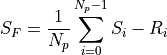
If the source has a radiance F, then the measured signal is equivalent to:

$S_F = F T_I - F T_S (N_p -1) = F T_E$

being T_I the integration time (ti), the time since the first productive read to the last productive read for a given pixel and T_S the time between samples (ts). T_E is the time between correlated reads $T_E = T_I - T_S (N_p - 1)$ .

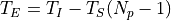The variance of the signnal is the sum of two terms, one for the readout noise:

$\mathrm{var}(S_{F1}) =\frac{2\sigma_R^2}{N_p}$

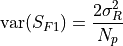
and other for the photon noise:

$\mathrm{var}(S_{F2}) = F T_E - F T_S \frac{1}{3}(N_p-\frac{1}{N_p}) = F T_I - F T_S (\frac{4}{3} N_p -1 - \frac{1}{3N_p})$

Parameters:

fowlerdata – Convertible to a 3D numpy.ndarray with first axis even
ti – Integration time.
ts – Time between samples.
gain – Detector gain.
ron – Detector readout noise in counts.
badpixels – An optional MxN mask of dtype ‘uint8’.
dtype – The dtype of the float outputs.
saturation – The saturation level of the detector.
blank – Invalid values in output are substituted by blank.

Returns:

A tuple of (signal, variance of the signal, numper of pixels used and badpixel mask.

Raises:

ValueError

numina.array.nirproc.ramp_array(rampdata, ti, gain=1.0, ron=1.0, badpixels=None, dtype='float64', saturation=65631, blank=0, nsig=None, normalize=False)

Loop over the first axis applying ramp processing.

rampdata is assumed to be a 3D numpy.ndarray containing the result of a nIR observation in folow-up-the-ramp mode. The shape of the array must be of the form N_s x M x N, with N_s being the number of samples.

Parameters:

fowlerdata – Convertible to a 3D numpy.ndarray
ti – Integration time.
gain – Detector gain.
ron – Detector readout noise in counts.
badpixels – An optional MxN mask of dtype ‘uint8’.
dtype – The dtype of the float outputs.
saturation – The saturation level of the detector.
blank – Invalid values in output are substituted by blank.

Returns:

A tuple of signal, variance of the signal, numper of pixels used and badpixel mask.

Raises:

ValueError

`numina.array.offrot` — Offset and Rotation

Fit offset and rotation

numina.array.offrot.fit_offset_and_rotation(coords0, coords1)

Fit a rotation and a translation between two sets points.

Fit a rotation matrix and a translation between two matched sets consisting of M N-dimensional points

Parameters:

coords0 ((M, N) array_like) –
coords1 ((M, N) array_lke) –

Returns:

offset ((N, ) array_like)
rotation ((N, N) array_like)

Notes

Fit offset and rotation using Kabsch’s algorithm [1] [2]

`numina.array.peaks` — Peak finding

Functions to find peaks in 1D arrays and subpixel positions

numina.array.peaks.peakdet.find_peaks_indexes(arr, window_width=5, threshold=0.0, fpeak=0)

Find indexes of peaks in a 1d array.

Note that window_width must be an odd number. The function imposes that the fluxes in the window_width /2 points to the left (and right) of the peak decrease monotonously as one moves away from the peak, except that it allows fpeak constant values around the peak.

Parameters:

arr (1d numpy array) – Input 1D spectrum.
window_width (int) – Width of the window where the peak must be found. This number must be odd.
threshold (float) – Minimum signal in the peak (optional).
fpeak (int) – Number of equal values around the peak

Returns:

ipeaks – Indices of the input array arr in which the peaks have been found.

Return type:

1d numpy array (int)

numina.array.peaks.peakdet.generate_weights(window_width)

Parameters:: window_width (int) – Odd number greater than 3, width of the window to seek for the peaks.
Returns:: Matrix needed to interpolate ‘window_width’ points
Return type:: ndarray

numina.array.peaks.peakdet.refine_peaks(arr, ipeaks, window_width)

Refine the peak location previously found by find_peaks_indexes

Parameters:

arr (1d numpy array, float) – Input 1D spectrum.
ipeaks (1d numpy array (int)) – Indices of the input array arr in which the peaks were initially found.
window_width (int) – Width of the window where the peak must be found.

Returns:

xc, yc – X-coordinates in which the refined peaks have been found, interpolated Y-coordinates

Return type:

tuple

numina.array.peaks.peakdet.return_weights(window_width)

Parameters:: window_width (int) – Odd number greater than 3, width of the window to seek for the peaks.
Returns:: Matrix needed to interpolate ‘window_width’ points
Return type:: ndarray

numina.array.peaks.detrend.detrend(arr, x=None, deg=5, tol=0.001, maxloop=10)

Compute a baseline trend of a signal

Parameters:

arr –
x –
deg –
tol –
maxloop –

`numina.array.recenter` — Recenter

Recenter routines

numina.array.recenter.centering_centroid(data, xi, yi, box, nloop=10, toldist=0.001, maxdist=10.0)

Computes centroid around point

Parameters:

data –
xi –
yi –
box –
nloop –
toldist –
maxdist –

Returns:

x, y, background, status, message
status is –
- 0: not recentering
- 1: recentering successful
- 2: maximum distance reached
- 3: not converged

`numina.array.robusfit` — Robust fits

Robust fits

numina.array.robustfit.fit_theil_sen(x, y)

Compute a robust linear fit using the Theil-Sen method.

See http://en.wikipedia.org/wiki/Theil%E2%80%93Sen_estimator for details. This function “pairs up sample points by the rank of their x-coordinates (the point with the smallest coordinate being paired with the first point above the median coordinate, etc.) and computes the median of the slopes of the lines determined by these pairs of points”.

Parameters:

x (array_like, shape (M,)) – X coordinate array. This array must be sorted.
y (array_like, shape (M,) or (M,K)) – Y coordinate array. If the array is two dimensional, each column of the array is independently fitted sharing the same x-coordinates. In this last case, the returned intercepts and slopes are also 1d numpy arrays. This array must be properly sorted to match the same order as the input X coordinate array.

Returns:

coef – Intercept and slope of the linear fit. If y was 2-D, the coefficients in column k of coef represent the linear fit to the data in y’s k-th column.

Return type:

ndarray, shape (2,) or (2, K)

Raises:

ValueError: – If the number of points to fit is < 5

`numina.array.stats` — Statistical utilities

numina.array.stats.robust_std(x, debug=False)

Compute a robust estimator of the standard deviation

See Eq. 3.36 (page 84) in Statistics, Data Mining, and Machine in Astronomy, by Ivezic, Connolly, VanderPlas & Gray

Parameters:

x (1d numpy array, float) – Array of input values which standard deviation is requested.
debug (bool) – If True prints computed values

Returns:

sigmag – Robust estimator of the standar deviation

Return type:

float

numina.array.stats.summary(x, rm_nan=False, debug=False)

Compute basic statistical parameters.

Parameters:

x (1d numpy array, float) – Input array with values which statistical properties are requested.
rm_nan (bool) – If True, filter out NaN values before computing statistics.
debug (bool) – If True prints computed values.

Returns:

result – Number of points, minimum, percentile 25, percentile 50 (median), mean, percentile 75, maximum, standard deviation, robust standard deviation, percentile 15.866 (equivalent to -1 sigma in a normal distribution) and percentile 84.134 (+1 sigma).

Return type:

Python dictionary

`numina.array.trace` — Spectrum tracing

numina.array.trace.traces.axis_to_dispaxis(axis): Obtain the dispersion axis from the spatial axis.

numina.array.trace.traces.trace(arr, x, y, axis=0, background=0.0, step=4, hs=1, tol=2, maxdis=2.0, gauss=1)

Trace peak in array starting in (x,y).

Trace a peak feature in an array starting in position (x,y).

Parameters:

arr (array) – A 2D array
x (float) – x coordinate of the initial position
y (float) – y coordinate of the initial position
axis ({0, 1}) – Spatial axis of the array (0 is Y, 1 is X).
background (float) – Background level
step (int, optional) – Number of pixels to move (left and rigth) in each iteration
gauss (bint, optional) – If 1 –> Gaussian interpolation method if 0 –> Linear interpolation method

Returns:

A nx3 array, with x,y,p of each point in the trace

Return type:

ndarray

class numina.array.trace.extract.Aperture(bbox, borders, axis=0, id=None): Spectroscopic aperture.

`numina.array.wavecalib` — Wavelength calibration

Automatic identification of lines and wavelength calibration

numina.array.wavecalib.arccalibration.arccalibration(wv_master, xpos_arc, naxis1_arc, crpix1, wv_ini_search, wv_end_search, wvmin_useful, wvmax_useful, error_xpos_arc, times_sigma_r, frac_triplets_for_sum, times_sigma_theil_sen, poly_degree_wfit, times_sigma_polfilt, times_sigma_cook, times_sigma_inclusion, geometry=None, debugplot=0)

Performs arc line identification for arc calibration.

This function is a wrapper of two functions, which are responsible of computing all the relevant information concerning the triplets generated from the master table and the actual identification procedure of the arc lines, respectively.

The separation of those computations in two different functions helps to avoid the repetition of calls to the first function when calibrating several arcs using the same master table.

Parameters:

wv_master (1d numpy array, float) – Array with wavelengths corresponding to the master table (Angstroms).
xpos_arc (1d numpy array, float) – Location of arc lines (pixels).
naxis1_arc (int) – NAXIS1 for arc spectrum.
crpix1 (float) – CRPIX1 value to be employed in the wavelength calibration.
wv_ini_search (float) – Minimum expected wavelength in spectrum.
wv_end_search (float) – Maximum expected wavelength in spectrum.
wvmin_useful (float) – If not None, this value is used to clip detected lines below it.
wvmax_useful (float) – If not None, this value is used to clip detected lines above it.
error_xpos_arc (float) – Error in arc line position (pixels).
times_sigma_r (float) – Times sigma to search for valid line position ratios.
frac_triplets_for_sum (float) – Fraction of distances to different triplets to sum when computing the cost function.
times_sigma_theil_sen (float) – Number of times the (robust) standard deviation around the linear fit (using the Theil-Sen method) to reject points.
poly_degree_wfit (int) – Degree for polynomial fit to wavelength calibration.
times_sigma_polfilt (float) – Number of times the (robust) standard deviation around the polynomial fit to reject points.
times_sigma_cook (float) – Number of times the standard deviation of Cook’s distances to detect outliers. If zero, this method of outlier detection is ignored.
times_sigma_inclusion (float) – Number of times the (robust) standard deviation around the polynomial fit to include a new line in the set of identified lines.
geometry (tuple (4 integers) or None) – x, y, dx, dy values employed to set the window geometry.
debugplot (int) – Determines whether intermediate computations and/or plots are displayed. The valid codes are defined in numina.array.display.pause_debugplot.

Returns:

list_of_wvfeatures – A list of size equal to the number of identified lines, which elements are instances of the class WavecalFeature, containing all the relevant information concerning the line identification.

Return type:

list (of WavecalFeature instances)

numina.array.wavecalib.arccalibration.arccalibration_direct(wv_master, ntriplets_master, ratios_master_sorted, triplets_master_sorted_list, xpos_arc, naxis1_arc, crpix1, wv_ini_search, wv_end_search, wvmin_useful=None, wvmax_useful=None, error_xpos_arc=1.0, times_sigma_r=3.0, frac_triplets_for_sum=0.5, times_sigma_theil_sen=10.0, poly_degree_wfit=3, times_sigma_polfilt=10.0, times_sigma_cook=10.0, times_sigma_inclusion=5.0, geometry=None, debugplot=0)

Performs line identification for arc calibration using line triplets.

This function assumes that a previous call to the function responsible for the computation of information related to the triplets derived from the master table has been previously executed.

Parameters:

wv_master (1d numpy array, float) – Array with wavelengths corresponding to the master table (Angstroms).
ntriplets_master (int) – Number of triplets built from master table.
ratios_master_sorted (1d numpy array, float) – Array with values of the relative position of the central line of each triplet, sorted in ascending order.
triplets_master_sorted_list (list of tuples) – List with tuples of three numbers, corresponding to the three line indices in the master table. The list is sorted to be in correspondence with ratios_master_sorted.
xpos_arc (1d numpy array, float) – Location of arc lines (pixels).
naxis1_arc (int) – NAXIS1 for arc spectrum.
crpix1 (float) – CRPIX1 value to be employed in the wavelength calibration.
wv_ini_search (float) – Minimum expected wavelength in spectrum.
wv_end_search (float) – Maximum expected wavelength in spectrum.
wvmin_useful (float or None) – If not None, this value is used to clip detected lines below it.
wvmax_useful (float or None) – If not None, this value is used to clip detected lines above it.
error_xpos_arc (float) – Error in arc line position (pixels).
times_sigma_r (float) – Times sigma to search for valid line position ratios.
frac_triplets_for_sum (float) – Fraction of distances to different triplets to sum when computing the cost function.
times_sigma_theil_sen (float) – Number of times the (robust) standard deviation around the linear fit (using the Theil-Sen method) to reject points.
poly_degree_wfit (int) – Degree for polynomial fit to wavelength calibration.
times_sigma_polfilt (float) – Number of times the (robust) standard deviation around the polynomial fit to reject points.
times_sigma_cook (float) – Number of times the standard deviation of Cook’s distances to detect outliers. If zero, this method of outlier detection is ignored.
times_sigma_inclusion (float) – Number of times the (robust) standard deviation around the polynomial fit to include a new line in the set of identified lines.
geometry (tuple (4 integers) or None) – x, y, dx, dy values employed to set the window geometry.
debugplot (int) – Determines whether intermediate computations and/or plots are displayed. The valid codes are defined in numina.array.display.pause_debugplot.

Returns:

list_of_wvfeatures – A list of size equal to the number of identified lines, which elements are instances of the class WavecalFeature, containing all the relevant information concerning the line identification.

Return type:

list (of WavecalFeature instances)

numina.array.wavecalib.arccalibration.fit_list_of_wvfeatures(list_of_wvfeatures, naxis1_arc, crpix1, poly_degree_wfit, weighted=False, plot_title=None, geometry=None, debugplot=0)

Fit polynomial to arc calibration list_of_wvfeatures.

Parameters:

list_of_wvfeatures (list (of WavecalFeature instances)) – A list of size equal to the number of identified lines, which elements are instances of the class WavecalFeature, containing all the relevant information concerning the line identification.
naxis1_arc (int) – NAXIS1 of arc spectrum.
crpix1 (float) – CRPIX1 value to be employed in the wavelength calibration.
poly_degree_wfit (int) – Polynomial degree corresponding to the wavelength calibration function to be fitted.
weighted (bool) – Determines whether the polynomial fit is weighted or not, using as weights the values of the cost function obtained in the line identification. Since the weights can be very different, typically weighted fits are not good because, in practice, they totally ignore the points with the smallest weights (which, in the other hand, are useful when handling the borders of the wavelength calibration range).
plot_title (string or None) – Title for residuals plot.
geometry (tuple (4 integers) or None) – x, y, dx, dy values employed to set the window geometry.
debugplot (int) – Determines whether intermediate computations and/or plots are displayed. The valid codes are defined in numina.array.display.pause_debugplot.

Returns:

solution_wv – Instance of class SolutionArcCalibration, containing the information concerning the arc lines that have been properly identified. The information about all the lines (including those initially found but at the end discarded) is stored in the list of WavecalFeature instances ‘list_of_wvfeatures’.

Return type:

SolutionArcCalibration instance

numina.array.wavecalib.arccalibration.gen_triplets_master(wv_master, geometry=None, debugplot=0)

Compute information associated to triplets in master table.

Determine all the possible triplets that can be generated from the array wv_master. In addition, the relative position of the central line of each triplet is also computed.

Parameters:

wv_master (1d numpy array, float) – Array with wavelengths corresponding to the master table (Angstroms).
geometry (tuple (4 integers) or None) – x, y, dx, dy values employed to set the window geometry.
debugplot (int) – Determines whether intermediate computations and/or plots are displayed. The valid codes are defined in numina.array.display.pause_debugplot.

Returns:

ntriplets_master (int) – Number of triplets built from master table.
ratios_master_sorted (1d numpy array, float) – Array with values of the relative position of the central line of each triplet, sorted in ascending order.
triplets_master_sorted_list (list of tuples) – List with tuples of three numbers, corresponding to the three line indices in the master table. The list is sorted to be in correspondence with ratios_master_sorted.

numina.array.wavecalib.arccalibration.match_wv_arrays(wv_master, wv_expected_all_peaks, delta_wv_max)

Match two lists with wavelengths.

Assign individual wavelengths from wv_master to each expected wavelength when the latter is within the maximum allowed range.

Parameters:

wv_master (numpy array) – Array containing the master wavelengths.
wv_expected_all_peaks (numpy array) – Array containing the expected wavelengths (computed, for example, from an approximate polynomial calibration applied to the location of the line peaks).
delta_wv_max (float) – Maximum distance to accept that the master wavelength corresponds to the expected wavelength.

Returns:

wv_verified_all_peaks – Verified wavelengths from master list.

Return type:

numpy array

numina.array.wavecalib.arccalibration.refine_arccalibration(sp, poly_initial, wv_master, poldeg, nrepeat=3, ntimes_match_wv=2, nwinwidth_initial=7, nwinwidth_refined=5, times_sigma_reject=5, interactive=False, threshold=0, plottitle=None, decimal_places=4, ylogscale=False, geometry=None, pdf=None, debugplot=0)

Refine wavelength calibration using an initial polynomial.

Parameters:

sp (numpy array) – 1D array of length NAXIS1 containing the input spectrum.
poly_initial (Polynomial instance) – Initial wavelength calibration polynomial, providing the wavelength as a function of pixel number (running from 1 to NAXIS1).
wv_master (numpy array) – Array containing the master list of arc line wavelengths.
poldeg (int) – Polynomial degree of refined wavelength calibration. Note that this degree can be different from the polynomial degree of poly_initial.
nrepeat (int) – Number of times lines are iteratively included in the initial fit.
ntimes_match_wv (int) – Number of pixels around each line peak where the expected wavelength must match the tabulated wavelength in the master list.
nwinwidth_initial (int) – Initial window width to search for line peaks in spectrum.
nwinwidth_refined (int) – Window width to refine line peak location.
times_sigma_reject (float) – Times sigma to reject points in the fit.
interactive (bool) – If True, the function allows the user to modify the fit interactively.
threshold (float) – Minimum signal in the peaks.
plottitle (string or None) – Plot title.
decimal_places (int) – Number of decimal places to be employed when displaying relevant fitted parameters.
ylogscale (bool) – If True, the spectrum is displayed in logarithmic units. Note that this is only employed for display purposes. The line peaks are found in the original spectrum.
geometry (tuple (4 integers) or None) – x, y, dx, dy values employed to set the window geometry.
pdf (PdfFile object or None) – If not None, output is sent to PDF file.
debugplot (int) – Debugging level for messages and plots. For details see ‘numina.array.display.pause_debugplot.py’.

Returns:

poly_refined (Polynomial instance) – Refined wavelength calibration polynomial.
yres_summary (dictionary) – Statistical summary of the residuals.

numina.array.wavecalib.arccalibration.select_data_for_fit(list_of_wvfeatures)

Select information from valid arc lines to facilitate posterior fits.

Parameters:

list_of_wvfeatures (list (of WavecalFeature instances)) – A list of size equal to the number of identified lines, which elements are instances of the class WavecalFeature, containing all the relevant information concerning the line identification.

Returns:

nfit (int) – Number of valid points for posterior fits.
ifit (list of int) – List of indices corresponding to the arc lines which coordinates are going to be employed in the posterior fits.
xfit (1d numpy aray) – X coordinate of points for posterior fits.
yfit (1d numpy array) – Y coordinate of points for posterior fits.
wfit (1d numpy array) – Cost function of points for posterior fits. The inverse of these values can be employed for weighted fits.

numina.array.wavecalib.peaks_spectrum.find_peaks_spectrum(sx, nwinwidth, threshold=0, debugplot=0)

Find peaks in array.

The algorithm imposes that the signal at both sides of the peak decreases monotonically.

Parameters:

sx (1d numpy array, floats) – Input array.
nwinwidth (int) – Width of the window where each peak must be found.
threshold (float) – Minimum signal in the peaks.
debugplot (int) – Determines whether intermediate computations and/or plots are displayed: 00 : no debug, no plots 01 : no debug, plots without pauses 02 : no debug, plots with pauses 10 : debug, no plots 11 : debug, plots without pauses 12 : debug, plots with pauses

Returns:

ixpeaks – Peak locations, in array coordinates (integers).

Return type:

1d numpy array, int

numina.array.wavecalib.peaks_spectrum.refine_peaks_spectrum(sx, ixpeaks, nwinwidth, method=None, geometry=None, debugplot=0)

Refine line peaks in spectrum.

Parameters:

sx (1d numpy array, floats) – Input array.
ixpeaks (1d numpy array, int) – Initial peak locations, in array coordinates (integers). These values can be the output from the function find_peaks_spectrum().
nwinwidth (int) – Width of the window where each peak must be refined.
method (string) – “poly2” : fit to a 2nd order polynomial “gaussian” : fit to a Gaussian
geometry (tuple (4 integers) or None) – x, y, dx, dy values employed to set the window geometry.
debugplot (int) – Determines whether intermediate computations and/or plots are displayed: 00 : no debug, no plots 01 : no debug, plots without pauses 02 : no debug, plots with pauses 10 : debug, no plots 11 : debug, plots without pauses 12 : debug, plots with pauses

Returns:

fxpeaks (1d numpy array, float) – Refined peak locations, in array coordinates.
sxpeaks (1d numpy array, float) – When fitting Gaussians, this array stores the fitted line widths (sigma). Otherwise, this array returns zeros.

Store the solution of a wavelength calibration

class numina.array.wavecalib.solutionarc.CrLinear(crpix, crval, crmin, crmax, cdelt)

Store information concerning the linear wavelength calibration.

Parameters:

crpix (float) – CRPIX1 value employed in the linear wavelength calibration.
crval (float) – CRVAL1 value corresponding tot he linear wavelength calibration.
crmin (float) – CRVAL value at pixel number 1 corresponding to the linear wavelength calibration.
crmax (float) – CRVAL value at pixel number NAXIS1 corresponding to the linear wavelength calibration.
cdelt (float) – CDELT1 value corresponding to the linear wavelength calibration.

Identical to parameters.

class numina.array.wavecalib.solutionarc.SolutionArcCalibration(features, coeff, residual_std, cr_linear)

Auxiliary class to store the arc calibration solution.

Note that this class only stores the information concerning the arc lines that have been properly identified. The information about all the lines (including those initially found but at the end discarded) is stored in the list of WavecalFeature instances.

Parameters:

features (list (of WavecalFeature instances)) – A list of size equal to the number of identified lines, which elements are instances of the class WavecalFeature, containing all the relevant information concerning the line identification.
coeff (1d numpy array (float)) – Coefficients of the wavelength calibration polynomial.
residual_std (float) – Residual standard deviation of the fit.
cr_linear (instance of CrLinear) – Object containing the linear approximation parameters crpix, crval, cdelt, crmin and crmax.

Identical to parameters.

update_features(poly): Evaluate wavelength at xpos using the provided polynomial.

class numina.array.wavecalib.solutionarc.WavecalFeature(line_ok, category, lineid, funcost, xpos, ypos=0.0, peak=0.0, fwhm=0.0, reference=0.0, wavelength=0.0)

Store information concerning a particular line identification.

Parameters:

line_ok (bool) – True if the line has been properly identified.
category (char) – Line identification type (A, B, C, D, E, R, T, P, K, I, X). See documentation embedded within the arccalibration_direct function for details.
lineid (int) – Number of identified line within the master list.
xpos (float) – Pixel x-coordinate of the peak of the line.
ypos (float) – Pixel y-coordinate of the peak of the line.
peak (float) – Flux of the peak of the line.
fwhm (float) – FWHM of the line.
reference (float) – Wavelength of the identified line in the master list.
wavelength (float) – Wavelength of the identified line estimated from the wavelength calibration polynomial.
funcost (float) – Cost function corresponding to each identified arc line.

Identical to parameters.

`numina.array.utils` —

Utility routines

numina.array.utils.coor_to_pix(w, order='rc')

Parameters:

w –
order –

numina.array.utils.coor_to_pix_1d(w): Return the pixel where a coordinate is located.

numina.array.utils.expand_region(tuple_of_s, a, b, start=0, stop=None): Apply expend_slice on a tuple of slices

numina.array.utils.expand_slice(s, a, b, start=0, stop=None): Expand a slice on the start/stop limits

numina.array.utils.extent(sl)

Parameters:: sl –

numina.array.utils.image_box(center, shape, box): Create a region of size box, around a center in a image of shape.

numina.array.utils.image_box2d(x, y, shape, box)

Parameters:

x –
y –
shape –
box –

numina.array.utils.slice_create(center, block, start=0, stop=None)

Return an slice with a symmetric region around center.

Parameters:

center –
block –
start –
stop –

numina.array.utils.wcs_to_pix(w)

Parameters:: w –

numina.array.utils.wcs_to_pix_np(w)

Parameters:: w –

numina.array — Array manipulation

numina.array.background — Background estimation

numina.array.blocks — Generation of blocks

numina.array.bpm — Bad Pixel Mask interpolation

numina.array.combine — Array combination

Combination methods in numina.array.combine

Extending generic_combine()

Simple combine method

A combine method with parameters

numina.array.cosmetics — Array cosmetics

numina.array.fwhm — FWHM

numina.array.imsurfit — Image surface fitting

numina.array.interpolation — Interpolation

numina.array.mode — Mode

numina.array.nirproc — nIR preprocessing

numina.array.offrot — Offset and Rotation

numina.array.peaks — Peak finding

numina.array.recenter — Recenter

numina.array.robusfit — Robust fits

numina.array.stats — Statistical utilities

numina.array.trace — Spectrum tracing

numina.array.wavecalib — Wavelength calibration

numina.array.utils —

`numina.array` — Array manipulation

`numina.array.background` — Background estimation

`numina.array.blocks` — Generation of blocks

`numina.array.bpm` — Bad Pixel Mask interpolation

`numina.array.combine` — Array combination

Combination methods in `numina.array.combine`

Extending `generic_combine()`

`numina.array.cosmetics` — Array cosmetics

`numina.array.fwhm` — FWHM

`numina.array.imsurfit` — Image surface fitting

`numina.array.interpolation` — Interpolation

`numina.array.mode` — Mode

`numina.array.nirproc` — nIR preprocessing

`numina.array.offrot` — Offset and Rotation

`numina.array.peaks` — Peak finding

`numina.array.recenter` — Recenter

`numina.array.robusfit` — Robust fits

`numina.array.stats` — Statistical utilities

`numina.array.trace` — Spectrum tracing

`numina.array.wavecalib` — Wavelength calibration

`numina.array.utils` —